The Gaussian quadrature for a square domain ([-1, 1] x [-1, 1]) can be conducted by a similar manner to 1D integration (see 1D Gaussian quadrature)
$\int \limits_{-1}^{1} \int \limits_{-1}^{1} g(\xi,\eta) d\xi\eta \approx \sum_{i=1}^{n} \sum_{j=1}^{n} g(\xi_i, \eta_j) w_i w_j$,
where $\xi$ and $\eta$ denotes the coordinate in horizontal and vertical direction, respectively. Theoretically, the number of integration points may be chosen different for $\xi$- and $\eta$- direction. However it is more convenient in practice to select the same $n$ number of integration points in each direction. The coordinates and weights of integration points along each direction is given in any FEM textbooks, and also in Wikipedia.
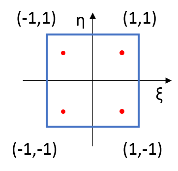
For example, if two Gauss points (i.e. integration points) are taken per direction (see Figure 1), the coordinates and weights are given in Table 1.
Table 1. Coordinates (in reference square) and weights of the Gauss points
| Point | $\xi$ | $\eta$ | weight |
| 1 (i = 1, j = 1) | $-\frac{\sqrt{3}}{3}$ | $-\frac{\sqrt{3}}{3}$ | $1 (=1 \times 1)$ |
| 2 (i =1, j = 2) | $-\frac{\sqrt{3}}{3}$ | $\frac{\sqrt{3}}{3}$ | $1 (=1 \times 1)$ |
| 3 (i =2, j = 1) | $\frac{\sqrt{3}}{3}$ | $-\frac{\sqrt{3}}{3}$ | $1 (=1 \times 1)$ |
| 4 (i =2, j = 2) | $\frac{\sqrt{3}}{3}$ | $\frac{\sqrt{3}}{3}$ | $1 (=1 \times 1)$ |
Integration on a convex quadrilateral domain can be easily transformed into integration on the square domain
$\int \limits_{\Omega} f(x, y) d \Omega = \int \limits_{-1}^{1} \int \limits_{-1}^{1} f(\xi,\eta) |\mathbf{J}| d\xi d\eta$,
where $ |\mathbf{J}| $ is the determinant of Jacobian matrix $\mathbf{J}$, which simply contains the derivatives of $x, ~y$ with respect to $\xi, ~ \eta$.
Using the same manner, it is straightforward to apply Gaussian quadrature for 3D domain.