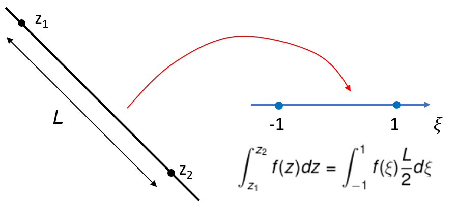
Integration on any straight line of length $L$ can be transformed into integration on the interval [-1, 1] by a simple transformation
$\int_{z_{1}}^{z_{2}} f(z) dz = \int \limits_{-1}^{1} \frac{L}{2} f(\xi) d\xi$
Note that the equation for transformation reads
$z = \frac{z_2 – z_1}{2} \xi + \frac{z_1 + z_2}{2}$
The integration on interval [-1,1] can be approximated by a summation.
$\int \limits_{-1}^{1} f(\xi) d\xi \approx \sum \limits_{i=1}^{n} w_{i} f(\xi_i)$
The above equation is the common form for numerical evaluation of integration. Following the Gaussian quadrature, the coordinates and weights of n integration points (or Gauss points) can be referred to Wikipedia.
The Gaussian quadrature provides exact solution if the integrand (i.e. the function to be integrated) takes the form of polynomials with the order up to 2n – 1. That is, if the integrand is a second order polynomials, 3 Gauss points are enough for exact calculation.
Note that an arbitrary curve can be approximated by a series of straight lines as illustrated in Figure 1. Therefore, integration on an arbitrary curve can be approximated as a sum of integration on straight lines.

The extension to integration on 2D domain is presented here